Computer Vision Laboratory (CVL)

Operations implemented in IPAPI

In this section we present some of the image processing operations developed in the project which have been implemented in the IPM of the helicopter.

As mentioned above, IPAPI has a CORBA interface which means that any other module of the system potentially can act as a client, creating and executing data flow graphs corresponding to various image processing operations. In practice, however, it is the TPEM who is the client using these services.

Detection and tracking of cars

Recall two of the high-level tasks mentioned in the IPM section, find vehicle and track vehicle. An example of how the processing is set up for these tasks is illustrated in figure 1.

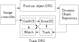
Figure 1: DFGs for identifying and tracking car objects. The ROI is chosen dynamically by sending requests to the Image Controller.

A typical result of the find vehicle operation is that a set of potential vehicles are identified. The terminal node of the corresponding data flow graph then exports the list of objects, acting as a CORBA client, to the DOR which is implemented as a CORBA server (right part of figure 2). At this point, the reasoning layers of the system examine the vision objects, e.g., check if their velocities are consistent with the direction of the road, or if their positions are on a road, or are consistent with predictions from earlier positions. If this is the case, a hypothesis can be made that this is an on-road object or a car object after additional reasoning and linkages are created and maintained between the object structures. A chronicle recognition service can then be called to identify various patterns of interest, i.e., simple sequences of events such as changing lane, stopping, turning, vehicle overtaking, etc.

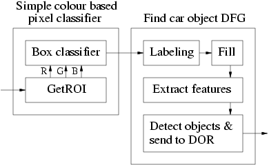
Figure 2: A simple DFG for finding car objects based on color classification. The left part classifies pixels according to their color, and the right part extracts blob shaped objects of a certain size, and sends them to DOR.

The linkage structures set up in the DOR are an important part of the signal to symbol conversions required for grounding qualitative symbol structures representing world objects such as vehicles to the sensory data associated with them. The grounding mechanism is always viewed as an ongoing process and the hypotheses made about such objects, such as an on-road object being a car, are always subject to change and must be monitored. If the sensory and qualitative data in a particular linkage structure changes too much and increases the uncertainty of the hypothesis, action must be taken to verify or retract the current hypothesis. This is often done by setting up a new image processing policy to acquire more information about the object in question or to refine the current values of features associated with the structure. Such refinement tasks require tight coupling between the TPEM, IPM and DOR.

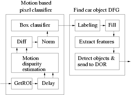
Figure 3: A more complex DFG for finding car objects based on motion estimation. The left part of figure 2 has been replaced by a DFG which estimates motion disparities.

Depending on the time available for the processing and the requirements for robustness, the TPEM can choose an appropriate algorithm and implement it in the IPM using the library of predefined nodes existing in IPAPI or pre-defined DFGs specialized for common tasks. For example, if the TPEM decides that it needs information about car objects with a minimum of delay, it can employ a method based on finding blobs of a certain color. This method assumes that the cars are of a distinct color relative to the background, and will of course not give a very reliable result, but can provide a result very fast, (left part of figure 2). On the other hand, if the TPEM requires the result to be more robust, it can employ a method for finding the cars based on motion, which uses more computational resources and takes a longer time to execute, see figure 3. Here, the color classification is replaced by a method which computes disparity estimates in a number of scales based on a polynomial expansion of the local signal [farneback02] [gfkn2002], see figure 4. The disparity estimate is iteratively refined at each finer scale, and the number of scales used (controlled by TPEM) has a direct consequence for the quality of the result, but also for the computation time.

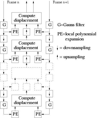
Figure 4: Expansion of the motion disparity estimation node in figure 3. The processing is made by a number of scale levels with identical operations. The coarsest level (at the bottom of the figure) computes a coarse disparity estimate, which is then refined by each succesive level.

Based on this type of processing, the TPEM can determine to start tracking a vehicle. This means that the IPM is reconfigured with a new processing graph implementing a suitable tracking method. With sufficient memory and processing power, multiple vehicles can be tracked simultaneously. The tracking operation continuously updates the object record in the DOR corresponding to the vehicle being tracked, while the TPEM monitors the tracking for possible tracking failure. One DFG used for tracking a vehicle is shown in the bottom of figure 1.

Camera position estimation

Another task which can be set up in the IPM is to continuously compute the position and orientation of the camera based on the motion in the image (a visual odometer) [forssen00]. Figure 5 illustrates the basic DFG for all the processing required for this task. The processing is based on tracking a set of points throughout the image sequence, and estimating a projective mapping given the motion of the points. Note that the DFG is cyclic because of the iterative estimation of the projective mapping. This capability can act as a backup or complement for the normal DGPS+INS system for navigation in cases where the system malfunctions.

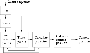
Figure 5: An overview of the visual odometer DFG.

The temporal aliasing in the camera image flow makes it necessary to use two-frame methods for motion or displacement estimation methods. For the visual odometer system, a method based on tracking of a sparse set of image regions was chosen. It typically keeps track of 50-60 local image regions over a longer time sequence. A region is automatically discarded when the matching value drops below a given threshold, and new regions to track are selected automatically by looking at local peaks in the second eigenvalue of the structure tensor.

Regions are tracked by template matching in response images from horizontal and vertical edge filters. Since edge filter responses are statistically sparse, and low-magnitude coefficients hardly affect the result at all, the templates can be pruned to use only 10% of the total number of coefficients. This results in a speedup of a factor above 3 in the total computations compared to full grey-scale correlation methods [forssen01b].

Last updated: 2012-06-01